There are over 2.07 billion monthly active Facebook Users worldwide as of Q3 2017. The most important aspect of the Facebook network is the social engagement between users. The more friends a user has, the more engaging the conversations become via comments on posts, messaging etc. If you’ve used Facebook fairly regularly, you must be knowing about the Friends Recommendation feature.
Facebook recommends a set of people that we can add as friends. Most of the times, these are people we’ve never heard of before. But still, Facebook thinks that we should add them.
The question is: how does Facebook come up with a set of recommendations for a specific person?
One way to do this is based on mutual friends. eg:- If a user A and C don’t know each other, but they have a mutual friend B, then probably A and C should be friends too. What if A and C have 2 mutual friends and A and D have 3 mutual friends? How will the ordering be for suggestions?
In this case, it seems pretty obvious to suggest D over C to A because they have more mutual friends and are more likely to get connected.
However, two people might not always have mutual friends, but they might have common 2nd-degree or 3rd-degree connections.
Nth Degree Connections
- A and B are friends.
(0 degree) - A and B are
1st-degreefriends means they have a mutual friend. - A and B are
2nd-degreefriends if they have a friend, who is a 1st-degree friend with the other person. eg:- A — C — D — B, then A and B are 2nd-degree friends. - Similarly, A and B are
Nth degreefriends if they have N connections in between. eg:- A — X1 — X2 — X3….. — XN — B.
Looking at this approach for the recommendation, we need to be able to find the degree of friendship that two given users share on Facebook.
Enter Graph Traversals
Now that we know how Friend Recommendations can be made, let’s restate this problem so that we can look at it from an algorithmic perspective.
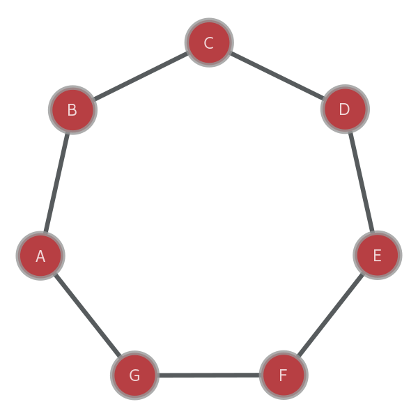
Let’s imagine an undirected graph of all the users on Facebook, where vertices V represent the users and edges E represent friendships. In other words: if users A and B are friends on Facebook, there is an edge between vertices A and B. The challenge is to find out the degree of connection between any two users.
More formally, we need to see the shortest distance between two nodes in an undirected, unweighted graph.

Consider two vertices in this undirected graph A and C. There are two different paths for reaching C:
- A → B → C and
- A → G → F → E → D →C
Clearly, we want to take the smallest path when trying to see the degree of connection between two people on the social network.
So far so good.
Before proceeding, let’s look at the complexity of this problem. As stated before, Facebook has around 2.07 billion users as of Q3 2017. That means our graph will have around 2.07 billion nodes and at least (2.07 billion — 1) edges (if every person has at least one friend).
This is a huge scale to solve this problem on. Additionally, we also saw that there might be multiple paths to reach from a given source vertex to a destination vertex in the graph and we want the shortest one to solve our problem.
We will look at two classic graph traversal algorithms to solve our problem:
- Depth First Search and
- Breadth First Search.
Depth First Search
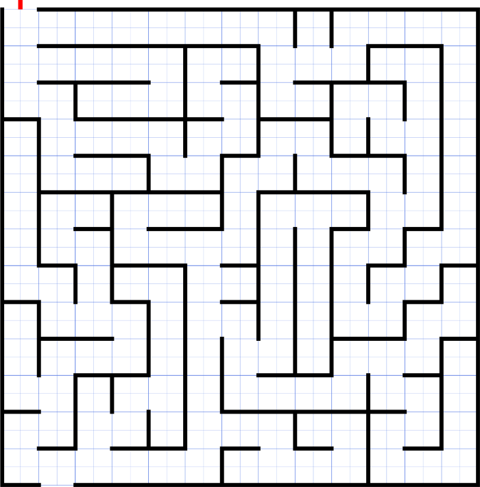
Imagine that you get stuck in a maze like this.

You have to get out somehow. There might be multiple routes from your starting position to the exit. The natural approach to getting out of the maze is to try all the paths.
Let’s say you have two choices at the point where you are currently standing. Obviously, you don’t know which one leads out of the maze. So you decide to make the first choice and move onwards in the maze.
You keep making moves and you keep moving forward and you hit a dead end. Now you would ideally want to try a different path, and so you backtrack to a previous checkpoint where you made one of the choices and then you try a new one i.e. a different path this time.
You keep doing this until you find the exit.
Recursively trying out a specific path and backtracking are the two components forming the Depth First Search algorithm (DFS).
If we model the maze problem as a graph, the vertices would represent the individual’s position on the maze and directed edges between two nodes would represent a single move from one position to another position. Using DFS, the individual would try all possible routes until the exit is found.
Here is a sample pseudo-code for the same.
1  **procedure** DFS(_G_,_v_):
2      label _v_ as discovered
3      **for all** edges from _v_ to _w_ **in** _G_.adjacentEdges(_v_) **do**
4          **if** vertex _w_ is not labeled as discovered **then**
5              recursively call DFS(_G_,_w_)
Time Complexity: O(V + E)
Breadth First Search
Imagine a contagious disease gradually spreading across a region. Every day, the people who have the illness infect new people they come into physical contact with. In this way, the disease is doing a sort of breadth-first-search (BFS) over the population. The “queue” is the set of people who have just been infected. The graph is the physical contact network of the region.
Imagine you need to simulate the spread of the disease through this network. The root node of the search is patient zero, the first known sufferer of the disease. You start off with just them with the disease, and no one else.
Now you iterate over the people they are in contact with. Some will catch the disease. Now iterate over all of them. Give the people they’re in contact with the disease too, unless they’ve already had it. Keep going until you’ve infected everyone, or you’ve infected your target. Then you’re done. That’s how breadth-first-search works.

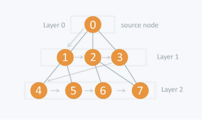
The BFS search algorithm explores vertices layer by layer starting at the very first vertex and only moving on to the next layer once all vertices on the current layer have been processed.
Here is a sample pseudo-code for BFS.
1   procedure BFS(G, v):
2       q = Queue()
3       q.enqueue(v)
4       while q is not empty:
5            v = q.dequeue()
6            if v is not visited:
7               mark v as visited (// Process the node)
8               for all edges from v to w in G.adjacentEdges(v) do
9                    q.enqueue(w)
For a deeper understanding of BFS, look into this article.
Time Complexity: O(V + E)
Shortest Paths
Let’s move forward and solve our original problem: finding the shortest path between two given vertices in an undirected graph.
Looking at the time complexities of the two algorithms, we can’t really make out the difference between the two for this problem. Both the algorithms will find a path (or rather the shortest path) to our destination from the given source.
Let’s look at the following example.

Suppose we want to find out the shortest path from the node 8 to 10. Let’s look at the nodes that DFS and BFS explore before reaching the destination.
DFS
- Process 8 → Process 3 → Process 1.
- Backtrack to 3.
- Process 6 → Process 4.
- Backtrack to 6.
- Process 7.
- Backtrack to 6 → Backtrack to 3 → Backtrack to 8.
- Process 10.
A total of 7 nodes are being processed here before the destination is reached. Now let’s look at how BFS does things.
BFS
- Process 8 → Enqueue 3, 10
- Process 3 → Enqueue 1,6
- Process 10.
Woah, that was fast! Just 3 nodes had to be processed and we were at our destination.
The explanation for this speedup that we can see in BFS and not in DFS is because DFS takes up a specific path and goes till the very end i.e. until it hits a dead end and then backtracks.
This is the major downfall of the DFS algorithm. It might have to expand 1000s of levels (in a huge network like that of Facebook, just because it selected a bad path to process in the very beginning) before reaching the path containing our destination. BFS doesn’t face this problem and hence is much faster for our problem.
Additionally, even if DFS finds out the destination, we cannot be sure that the path taken by DFS is the shortest one. There might be other paths as well.
That means that in any case, for the shortest paths problem, DFS would have to span the entire graph to get the shortest path.
In the case of BFS, however, the first occurrence of the destination node ensures that it is the one at the shortest distance from the source.
A fun problem
So far we discussed the problem of Friends Recommendation by Facebook and we boiled it down to the problem of finding the degree of connections between two users in the network graph.
Then we discussed two interesting Graph Traversal algorithms that are very commonly used. Finally, we looked at which algorithm performs the best for solving our problem.
Breadth First Search is the algorithm you want to use if you have to find the shortest distance between two nodes in an undirected, unweighted graph.
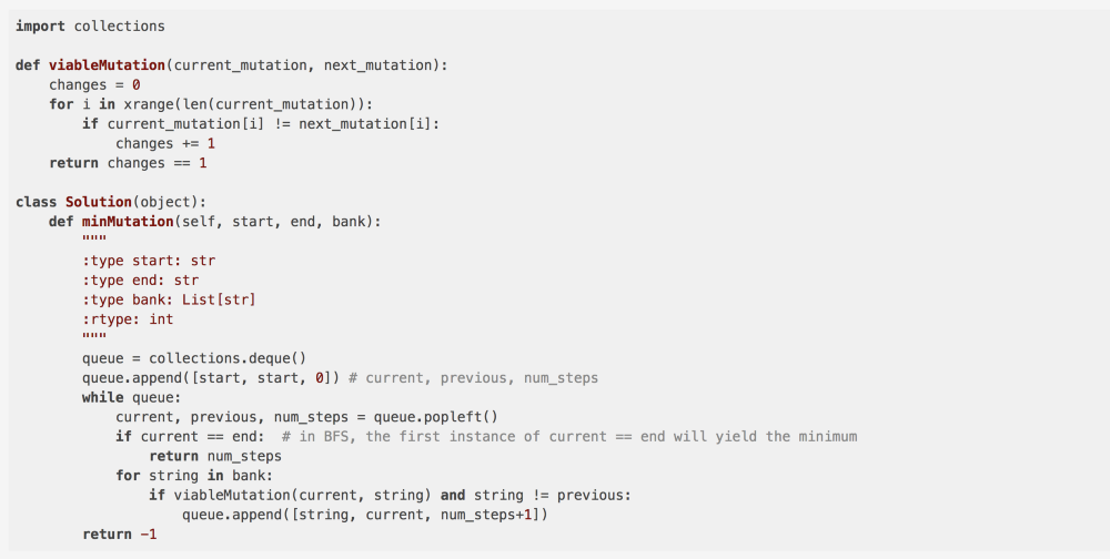
Let’s look at this fun problem to depict the difference between the two algorithms.
Assuming that you’ve read the problem statement carefully, let’s try and model this as a graph problem in the first place.
Let all possible strings become nodes in the graph and we have an edge between two vertices if they have a single mutation between them.
Easy, right?
We are given a starting string (read source vertext) eg:- “AACCGGTT” and we have to reach the destination string (read destination vertex) “AACCGGTA” in minimum number of mutations (read minimum number of steps) such that all intermediate strings (nodes) should belong to the given word bank.
Try and solve this problem on your own before looking at the solution below.

If you try to solve it using DFS, you will surely come up with a solution, but there is a test case(s) that will exceed the allotted time limit on the LeetCode platform. That’s because of the problem described before as to why DFS takes so long (process 7 nodes as opposed to 3 in BFS) to reach the destination vertex.
Hope you got the main idea behind the two main graph traversals, and the difference between them when the application is shortest paths in an undirected unweighted graph.
Please recommend (❤) this post if you think this may be useful for someone!

Leave a comment