The Perfect Programming Interview Problem

Telephone screening interviews are a bit easier than the traditional onsite whiteboard interviews. The whiteboard interviews involve a whole lot of pressure and anxiety due to the lack of a code editor to code on. The thing that these interviews do have in common is the kind of skills they test.

Usually, a programming interview will involve one programming challenge. The candidate has to work on it for the duration of the interview. The time allotted is usually 30–35 minutes. The first 10 minutes are taken up by introductions and other things.

Given a programming problem, the interviewer usually wants the candidate to:

Give a Working Solution Come up with a working solution for the problem. This can be a brute force solution to start with. The criterion is that the candidate should be able to code up a syntactically correct program for the algorithm in that small time frame.
Ask Clarification Questions Ask questions to clarify things that were intentionally left out.
→ What’s the size of the input?
→ How many numbers can be in the array?
→ What is the alphabet size for the string given?
→ Can we use extra memory?
→ Can we modify the given input or is that read-only?
Syntactically Correct Code Once the interviewer is convinced of the solution that the candidate is describing, they are expected to write a working solution for the problem. In a whiteboard interview this solution is to be written on the whiteboard. The whiteboard obviously doesn’t have any syntax correction! That’s what makes it really hard.
Come up with better solutions If you only present a brute force solution to the interviewer to break the awkward silence, they will more often than not ask you to come up with a better solution. Unless it’s your luck day and the interviewer is convinced with the solution you proposed 😉. The kind of follow up questions they generally ask are:
→ Can you come up with a better solution? O(logn) → O(n)
→ Can you make your solution space efficient? O(1) space.
Edge Cases Even if you were able to come up with an optimal working solution for the problem, it is possible that you missed out on a few edge cases. You may have missed out on a few scenarios that don’t change the algorithm. They may affect the implementation. A candidate is expected to do extensive dry runs with the code after writing it. You are expected to try out a few test cases to find any issues they might have left in their code.
Complexity Analysis If there is still time remaining in your interview and the interviewer seems to be satisfied with the code you came up with, they might ask you about the time and space complexity of your solution. Hence, complexity analysis is also a critical skill set required to crack these programming interviews.

Yes, it is indeed overwhelming.

This post is not really about tips and tricks about preparing for and attempting a programming interview. There are a lot of good posts out there for this.

I recently came across a programming problem that I had to solve within a time span of 1 hour. It was a part of a programming contest being held on Leetcode. I found this problem to be a great candidate to be asked in a programming interview.

I will go through the problem in detail here and discuss my reasons for why this is a good interview problem. I will do my best to try and relate it to the points mentioned before.

🐍 Let’s Play Snakes and Ladders

This question was a part of a recent weekly programming contest held on LeetCode. It’s a 1.5 hour contest with 4 programming challenges of varying difficulty.

This problem was marked as a medium difficulty problem. Being able to solve it during the timeframe is a big thing as you will realize after going through the article.

It’s a big question and I would definitely urge you to go through it before reading on.

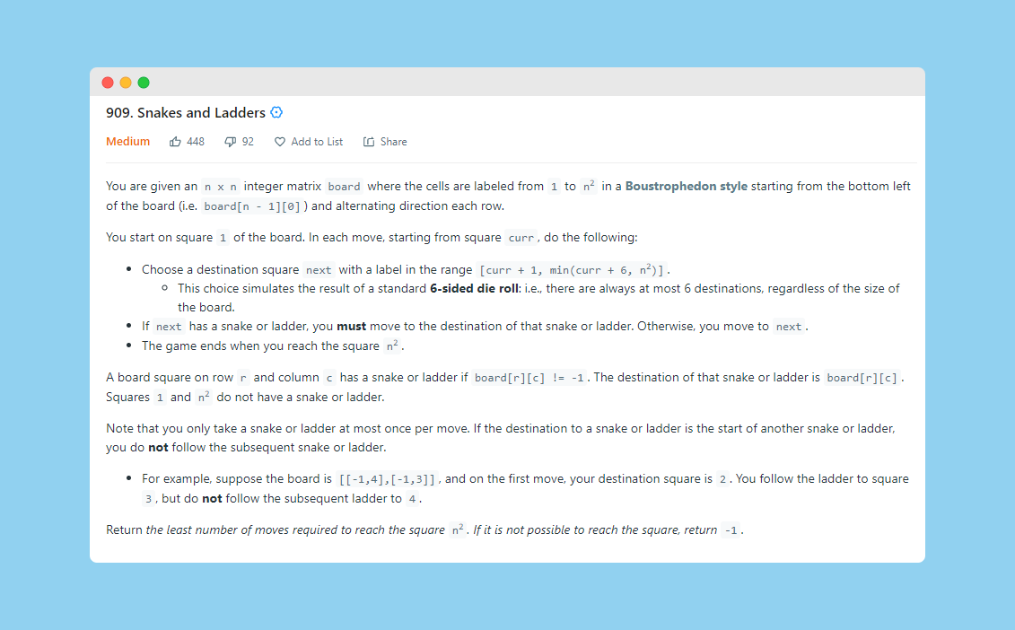
The part of the problem that I want you to focus on is the following:

Return the least number of moves required to reach square N*N. If it is not possible, return -1.

Looks like a typical Dynamic Programming problem

Or is it?

If you have been practicing dynamic programming problems for a while, it should be a no-brainer that problem statements similar to the one above usually employ the dynamic programming paradigm.

The reason we say this is because for a problem to be solvable using dynamic programming, it should have certain characteristics.

The problem should be breakable into smaller subproblems. The subproblems can be used to solve the main problem. Optimal solutions to subproblems should help us find the optimal solution to the main problem. This means a problem should be solvable recursively.
The second most important property is that of overlapping subproblems. Essentially, what dynamic programming does for us is that it helps us reuse optimal solutions for subproblems. In case we have multiple recursion paths with overlapping subproblems, we should only calculate answers for them once. Then onwards reuse them. This is the caching part of dynamic programming.

The reason why this problem fits the bill for dynamic programming is because of the following components of the problem:

We have a grid where each cell has a specific number. That number can help us define the state of a dynamic programming solution.
At every cell in the grid, we have 6 options available. These represent the 6 dice values that we can possibly get on playing snakes and ladders. Naturally, these 6 steps help us transition from one state to another state. This represents the “breakable into subproblems” part of the dynamic programming requirements.
Since we can break the problem down into smaller subproblems, we already have one requirement satisfied. If you think carefully, it is possible to reach the same cell on the grid multiple times via different routes. Let us look at two possible ways of reaching the cell value 22 starting from 1 .

Route Followed: 1 → 4 → 10 (Snake Up!) → 22

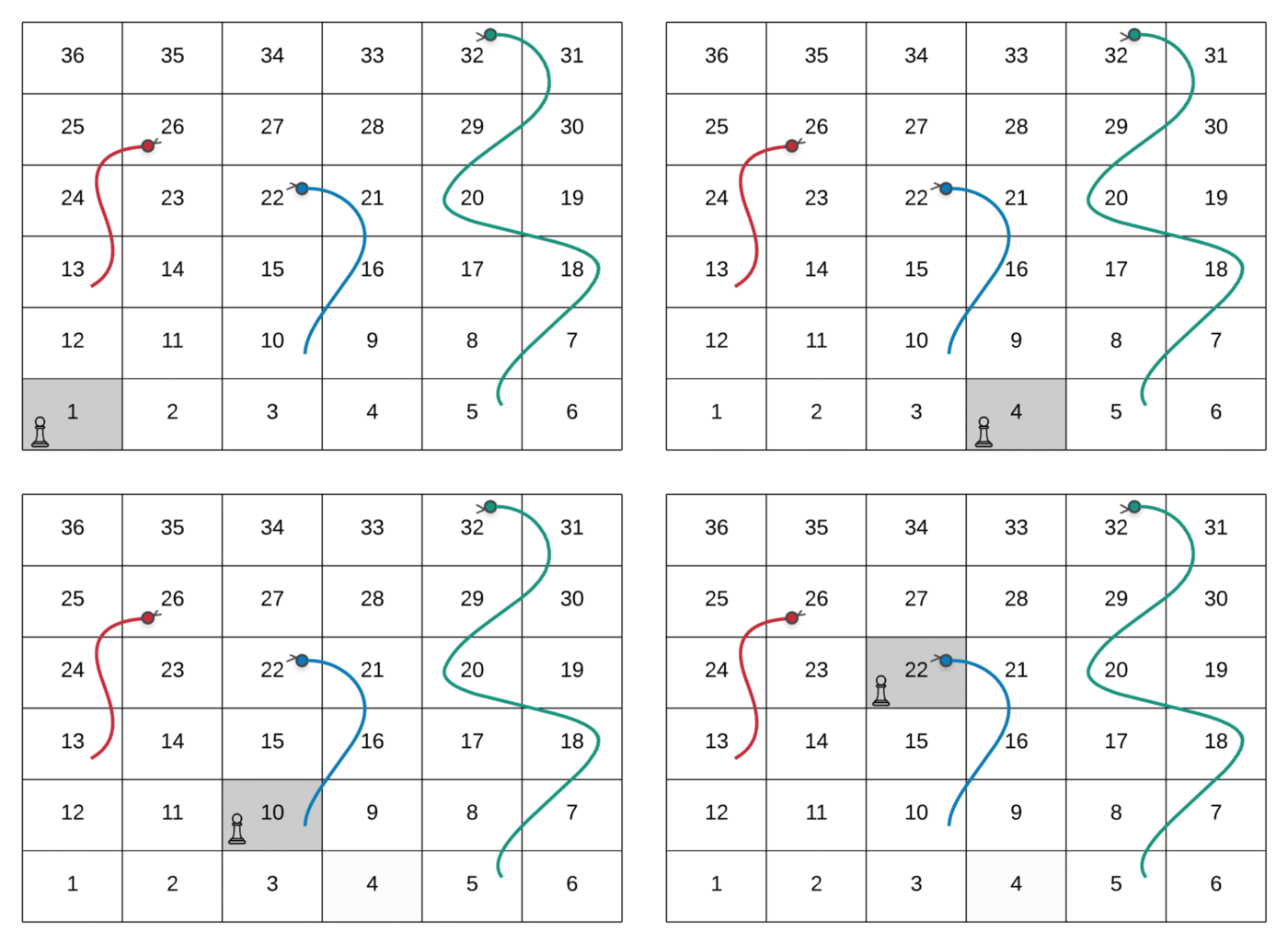
The path followed by the player in the above GIF is as follows:

--> Start at the node marked 1  
--> Dice value 3, hence move to node marked 4  
--> Dice value 6, hence move to node marked 10  
--> Since there was a snake at node 10, move to its head and hence the node valued **22**.

Route Followed: 1 → 4 → 9 → 14 → 17 → 22

The path followed by the player in the above GIF is as follows:

--> Start at the node marked 1  
--> Dice value 3, hence move to node marked 4  
--> Dice value 5, hence move to node marked 9  
--> Dice value 5, hence move to node marked 14  
--> Dice value 3, hence move to node marked 7  
--> Dice value 5, hence move to node marked **22**

As we can see from the two paths above in a sample snakes and ladders grid, there are two ways of reaching the node valued 22 . There are a lot of other ways as well. To put across the point of overlapping subproblems, the two shown here are enough.

Now that we know a single cell defines the state of our dynamic programming solution and there are multiple ways of reaching the same cell, this implies that our second requirement for a dynamic programming problem is also satisfied i.e. overlapping subproblems. Once having calculated the answer for a given subproblem, it shouldn’t be computed again. It should just be re-used.

Let us now look at a formal dynamic programming formulation for this problem.

dp[i] = Minimum number of steps from cell(i) to reach the destination cell.
dp[i] = min(dp[i + 1], dp[i + 2], ... dp[1 + 6])  
We have to choose the move that gives the minimum number of steps.

The above formulation looks pretty clean and we can proceed with it.

However, there’s a major flaw in the above formulation. 😉

The way we have modeled our problem here is something that will continue till the end of the article. So, let us first define the model of our problem. Then continue with describing the flaw in the dynamic programming approach.

Graph Model

We can consider each of the cells in our snakes and ladders grid as a node in a graph. The six possible moves that a player can make from a given cell represent the edges. These edges are directed edges. A move that takes us from cell i to cell j , doesn’t necessarily take us back from cell j to cell i . So, for the problem formulation we have:

A Graph G(V, E)
Each cell in our snakes and ladders grid represents a node in the graph. Naturally, there are N² nodes in the graph.
Every move from cell i to cell j represents a directed edge in the graph from node i to node j .
Since, for every cell in the grid, we have at most 6 moves, this means the total number of edges in our graph would be 6N².

Let’s consider a small grid and its corresponding graph for more clarity.

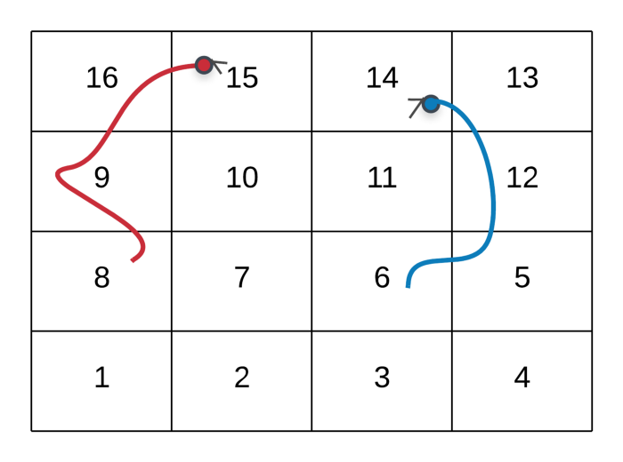
And the corresponding graph for this grid would be.

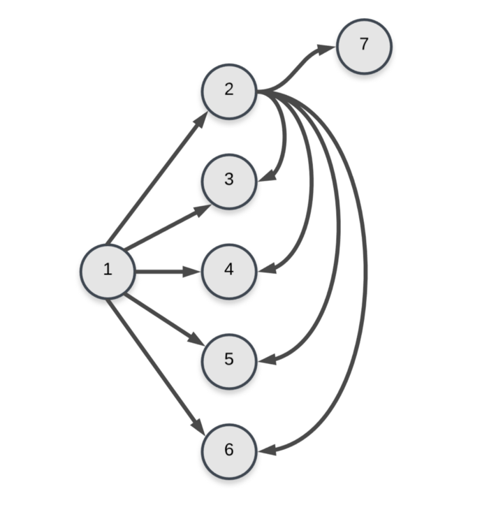
Edges for nodes 1 and 2 in the graph. As you can imagine, the graph becomes complicated very quickly because of the number of edges. There should be 4 * 4 * 6 = 96 edges in total in the graph since we have 16 nodes and each of them will have 6 edges in total. But, the final nodes 11–16 will have fewer edges. e.g. 11 will have just 5 edges. Similarly, 16 will have 0 edges. Hence, total edges will be 96 — (1 + 2 + 3 + 4 + 5 + 6) = 75.

The Flaw in our DP formulation

Now that we have defined our graphical model for the problem, we can look at the flaw in our dynamic programming formulation. The formulation we looked at was the following:

dp[i] = Minimum number of steps from cell(i) to reach the destination cell.
dp[i] = min(dp[i + 1], dp[i + 2], ... dp[1 + 6])  
We have to choose the move which gives the minimum number of steps.

If there were no snakes involved in the problem, then the above formulation would have been complete in itself. The problem induced by the snakes is that of loops in our graph. A snake can bring us back to an already visited state in our graph.

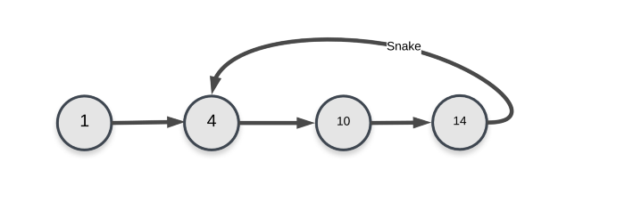
Loop introduced by snakes in the graph representation.

The problem this creates in our formulation is we can’t really consider a single cell in the grid to define the state of our dynamic programming formulation.

Let’s see why that is the case via an example and then we will see how to fix this problem by a different formulation.

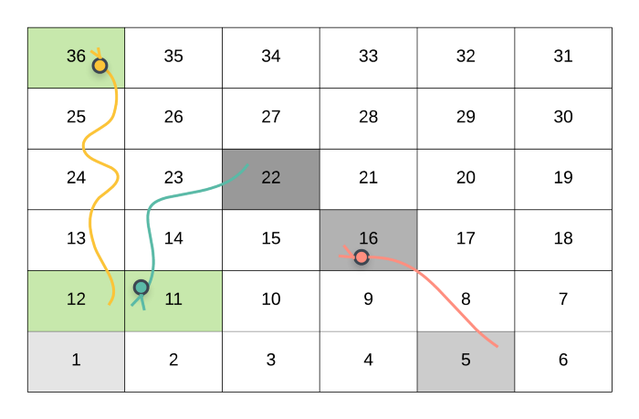
The player moves from cell 1 to 22 and follows the path 1 → 5 → 16 (Snake Up!) → 22.

This is one of the possible routes of reaching the cell 36 starting from the initial cell 1.

Suppose that we want to find out the shortest number of steps to take from cell 22 to reach the destination cell 36 . In the above case, the player went from 1 --> 5 --> 16 (Snake Up!) --> 22 . As we can see in the above figure, the player will come down to the cell 11 due to the snake. Then take one step ahead i.e. to cell 12. Finally, take the snake up to the destination cell 36 . This is just 1 step.

Following the snake from 22 --> 11 and from 12 --> 36 is not really a move. The actual move is from 11 --> 12 . Hence, the minimum number of steps required to move from 22 to 36 is 1.

Now consider the following state of the grid when the user had reached 22 .

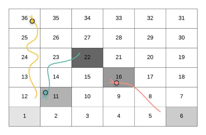
The player moves from cell 1 to 22 and follows the path 1 → 6→ 11 → 16 → 22.

The above scenario is also possible during recursion. In this case, when the player reaches the cell 22, they don’t have 6 options in front of them. The reason for that is, the cell 22 is the starting point for a snake. If a cell is a starting point for a snake, then it has to be followed to its head. The player will end up landing in cell 11 which has already been visited. This is a loop in our recursion. Since we cannot make any other move from cell 22 , there is no way of finding out the minimum number of steps from 22 to 36 .

The problem is:

A cell alone cannot represent the state of our dynamic programming formulation. We also need to keep track of the cells visited prior to the one at hand. A combination of these two would define a unique state in our DP formulation.

Updated DP formulation

The updated DP formulation, as mentioned before will have to take into account the visited cells and the current cell where the player is at.

Since, the state of a dynamic programming problem is generally used as a key to a cache that stores the results for various states (memoization), simply keeping a dictionary or a set of visited cell nodes is not feasible. These data structures are not hashable.

An alternative approach which can be adopted is bit-masking. We can make use of a bit-mask to mark the cells of the grid that a user has already visited before visiting a particular cell.

Let’s consider if this is even a feasible approach to follow. So, for a grid size of 20-by-20 , there would be 400 cells and we would need a bit-mask of 400 bits. Each of these bit values would represent if that particular cell is already visited or not during recursion. Since each of the bits can have two different values: 0 and 1 , there are 2^400 possible grid states. Multiplying it with 400 since we also need the current cell, we get a whopping (2^400 * 400).

Such a huge number of possible states will not work out and is not tractable at all. This is the reason that we have to move on from a dynamic programming solution to something else because of the sheer number of states in the problem formulation.

Breadth First Search to the Rescue! ⛑

Let’s try and formulate the problem in a slightly different manner. We already said that the cells in our grid represent the nodes in a graph. The 6 possible moves represent the directed edges to other nodes in the graph.

We want to find the minimum number of moves of reaching the destination starting from the initial point on the grid. This boils down to finding the shortest path in an unweighted graph.

You can either say this graph is unweighted, or you can say that all the edges are of equal weights. Hence the weights can be ignored. Finding the shortest path in an unweighted graph is a pretty standard problem. The most standard algorithm for solving it is the breadth first search algorithm.

We don’t need any special state in our graph for breadth first search like we needed in the case of dynamic programming. We can definitely have multiple ways of reaching a particular node from the starting position. However, the first route that is discovered in the breadth first search algorithm is the shortest one. That is the basis for the algorithm.

That means the first time we encounter a node/cell during our search, the number of moves performed till then would be the minimum number of moves required to get to that state/cell/node from the starting position.

After that if we encounter the same node again, we can simply ignore it. We would already have the shortest path to that node by then. This ensures that we don’t process any node of the graph more than once in breadth first search.

The breadth first search algorithm makes use of the queue data structure. The queue contains the nodes of the graph at a particular level at any point in time. Since we will only process each node exactly once, the maximum possible size of the queue can be O(N). That’s the upper bound on the size of the queue. This approach to the problem is very tractable and is in fact the optimal way of doing it.

Let’s look at the pseudo-code for the algorithm that we just proposed for this problem. Then we will look at the implementation for the same.

1. Initialize a queue for the BFS algorithm. Let's call it "Q".  
2. Add the first cell to the Q. Note that we also need to keep track of the level of nodes in our graph. The level will tell us the minimum number of moves made to reach a specific node. The level for the initial node would be 0.  
3. Process until the Q becomes empty.  
    a. Remove the front element of the Q. Let's call it "node".  
    b. For each of the 6 possible moves from "node", add the ones that have not been processed before, to the Q.  
4. If we encounter the destination node during the processing, simply return the level value at that point.

There are a lot of interesting points that we should address before looking at the implementation. These are from my own attempt at the problem. Some of these might seem too simple to have been mentioned. I wanted to put across all these cases. They are important to they way you write the code for this algorithm we discussed.

Cell Value to Row and Column Mapping 👺

The first of these points that is important to think about is the mapping from the cell values to the actual row and column numbers.

Remember, we are given a grid of some values and each cell of the grid has a numbering. The numbering system is written boustrophedonically from bottom starting from the bottom left of the board, and alternating direction each row.

The way the implementation has been done here initially is by considering the actual row and column numbers and then somehow using them to progress in the grid.

According to the problem, if a cell contains a snake, then the value in that cell is the destination cell where the player would land. We need to map the destination cell value to the corresponding row and column number.

The movement for the row is always easy. We either move in different columns in the same row or we can shift one row up. That’s it for the row.

As far as the column is concerned, there are two possible directions of movement. The question is especially tricky. The numbering of the cells alternates from one row to another. The movement within a row (for the various moves) will also have alternating directions in alternating rows e.g. for a 6-by-6 grid, the movement will be to the right for the bottom row and it will be to the left in the second last row.

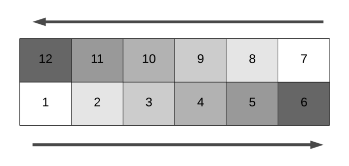
For a 6-by-6 matrix, the row number 5 (considering a 0-based indexing of the matrix rows and columns) would be the one containing cells from 1 .. 6 and the row number 4 would contain the cells from 7 .. 12 .

This means, for the even numbered rows, the direction is to the left. For the odd numbered rows, the direction is to the right. However, This mapping gets reversed when N is odd. Consider the scenario in a 5-by-5 matrix.

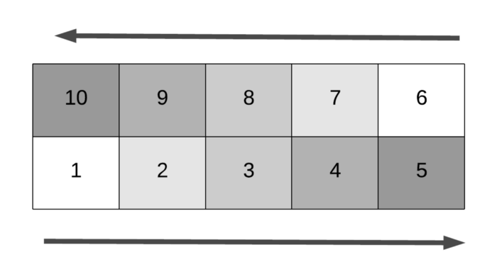
The last row in this matrix is 4 and that row has a direction to the right. This means, in these cases, the even numbered row has a direction to the right. The odd numbered row has a direction to the left.

Implementation wise, we can use something like the following.

even_direction = 1 if N % 2 != 0 else -1  
direction = even_direction * (1 if row % 2 == 0 else -1)

In our implementation, we consider a value of 1 for a direction to the right and a value of -1 for representing a direction to the left. The reason for this is the simplicity it induces in simulating movement. We can simply do something like:

for move in range(6):  
     new_cell = cell[r][c + direction]

The c + direction would either go towards right or left. This is because the value of direction will either be 1 or -1 depending upon the value of N .

Now we can look at the mapping of a cell value to the corresponding row and column indices.

Note that the following code is only to be executed when we find a snake in one of the cells. board[row][col] will contain a -1 to represent a normal cell. The following code is executed when a snake is found i.e. board[row][col] != -1

(1) value = board[row][col]  
(2) snake_dest_row = N - (value / N) - 1  
(3) new_direction = even_direction * (1 if snake_dest_row % 2 == 0 else -1)  
(4) snake_dest_column = (value % N)  
                          
(5) if new_direction < 0:  
(6)    snake_dest_column** = N - 1 - snake_dest_column  
                          
(7) next_cell = (snake_dest_row, snake_dest_column)

Line 1

Gives us the value stored at the current cell. The current cell is represented by row and col .

Line 2

Using the value stored in the cell we find the row where that cell would be located. Remember, the value represents the cell we need to move the player to since they encountered a snake.

Line 3

Since we figured out the row where the new cell (destination cell) would be located, we can also figure out the direction of cells in that particular row. We discussed directions to the right and left depending upon the value of N, above.

Line 4, 5 and 6

Represents the offset for finding out the column value. For a row which has a direction going to the right, the offset itself will represent the column index. If the direction is to the left, then the offset will be from the right. We find the column index using N — snake_dest_column — 1 .

Problematic Cell Values 😠

As mentioned before, the cells either contain -1 or they contain a snake. The way a snake is represented is by a cell value that represents the destination cell that a player will reach by following that snake.

So, while handling the snake case, we need to be able to get the row and column number where the corresponding cell will be located.

We saw in the previous section the way we can do that. There’s a small mistake in the code, however.

Consider the scenario where we have a 4-by-4 grid. A particular cell contains a snake that takes the player to (or whose destination cell is) 8 . Let’s see the corresponding row and column values that we get by using the code above.

value = 8  
even_direction = -1  
snake_dest_row = 4 - (8 / 4) - 1 = 1  
new_direction = -1 * (-1)  = 1
snake_dest_column = 8 % 4 = 0
next_cell = (1, 0)

Clearly, this is not the correct cell. The correct cell representing the value 8 is (2, 0) and not (1, 0) . The way we fix this is by not considering the value as it is but by subtracting 1 from it. Then this problem doesn’t arise.

value = board[row][col] - 1

Making one move per Snake 🐍

One of the last important components of the implementation is adhering to the rule mentioned in the problem statement which states that “you only take a snake or ladder at most once per move”. If the destination to a snake or ladder is the start of another snake or ladder, you do not continue moving.

The way BFS works is, we process the node currently popped from the queue by looking at its adjacency list. Then consider all the nodes that have not been processed yet and then add them to the queue.

So, for a given cell, there would be 6 adjacent nodes. Except for some cases where it’s not possible to have 6 moves in all. We have to consider all them and add the ones not processed yet to the queue.

No special handling is required for the moves that land up in cells that don’t contain a snake. So, all we do in this case is:

if board[row][col + direction] == -1:  
    process it normally

In case the move we make lands us with a snake, instead of considering / processing the node where we are after the move, we consider the snake’s destination cell and add that to the queue instead if it was not processed before. Let’s consider an example for this.

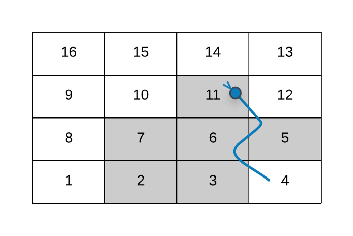
The 6 moves when the player is at the cell 1

As you can see in the figure above, we don’t consider the node 4 when processing the 6 moves corresponding to the cell 1 . Instead we consider the eventual destination for 4 i.e. 11 .

If suppose there were a snake from 11 to some other node, then we will not process that. We already processed one snake move from 4 to 11 . There cannot be a continuation of snake moves here. That is an important thing to note.

Let’s look at the implementation that brings all these ideas together.

Can we get rid of the “direction” thingy? 😬

It turns out there’s a simpler way of doing what is accomplished using the even_direction variable above.

Essentially we want to know, given a row number, what is the direction of cells in it. Is it towards the right or towards the left?

The reason we need this information is because that helps us decide the final column number when we encounter a snake.

Instead of relying on the even_direction variable, we can use a simple check like the following:

if N % 2 != row % 2:  
   direction = right  
else  
   direction = left

This covers all of the cases for us. Remember, the direction for a row depends upon the value of N.

N is even and row is even, then N % 2 == row % 2 and hence the direction will be towards left.
N is even and row is odd, then N % 2 != row % 2 and hence the direction will be towards right.
N is odd and row is odd, then N % 2 == row % 2 and hence the direction will be towards left.
N is odd and row is even, then N % 2 != row % 2 and hence the direction will be towards right.

Mapping the other way around

In the above implementation, we worked with row and column numbers. Then mapped a cell value to a row and column number whenever required (in case of snake that is). We can also solve this problem by working the other way around.

It’s much simpler to work with cell numbers instead. Starting from 1 and for every cell we have to consider the next 6 cells.

All we would have to do is then map those cell values to the corresponding row and column numbers (again, to check the presence or absence of any snakes). We already saw how to do that in the above implementation as well.

This shortens the code. The solution I explained above is the one I came up with when thinking about the problem. I wanted to explain it as it is to make things clearer. This might not be the best way to go about writing the code for the algorithm describer. It helps describe all the caveats.

Why again this is the best programming interview problem?

You might be lured towards a dynamic programming based solution (like I was 😛). In that case you need to reason and get out of that loophole. DP doesn’t work here.
Coming up with a BFS based approach here is super critical. A good grasp of your graph based algorithms is necessary. The important thing is mapping the problem to finding shortest paths in unweighted graph.
Writing the code for mapping cell values to corresponding row and column numbers can be super confusing especially under time constraints. It’s not a big piece of code but you need to be able to think it through properly.
Handling the edge case where we get incorrect mapping if we consider cell values as it is. We had to subtract 1 from the cell value before mapping it to the corresponding row and column. Failure to do this will give incorrect results.
Writing correct, working code during time constraints is also a tough-ish task. You really need to keep your cool.

All in all, this problem tests a lot of different aspects of programming and thinking ability of a programmer. I feel that is one of the most important aspects to test during such interviews.

Not that these interviews are the best way to hire the candidates. Since they exist, this problem brings out a lot of different qualities that interviewers look for in candidates.

If you found the article to be useful, do share it as much as possible 🚀

Share on

Twitter Facebook LinkedIn