That’s a weird looking title, that probably doesn’t make sense right now. But trust me, this is a pretty long post and is really fun!
What is Backtracking ?
Backtracking is a standard problem solving technique based on recursion.
A backtracking algorithm tries to build a solution to a computational problem incrementally. Whenever the algorithm needs to decide between multiple alternatives to the next component of the solution, it simply tries all possible options recursively.
Depth First Search (DFS) uses the concept of backtracking at its very core. So, in DFS, we basically try exploring all the paths from the given node recursively until we reach the goal. After we explore a particular branch of a tree in DFS, we can land up in two possible states.
- We found the goal state in which case we simply exit.
- Or, we did not find the goal state and we hit a dead end. In this scenario, we backtrack to the last checkpoint and we then try out a different branch.
For detailed introduction to the Depth First Search Algorithm, go through one of my other articles here and for backtracking, head over here.
Now that we are all pros in backtracking and recursion, let’s see what do “Queens” have to do with all this.
The Famous N-Queens Problem
Positioning queens on a chess board is a classical problem in mathematics and computer science.
The Queen’s Puzzle (aka the eight queens puzzle), was originally published in 1848. It involves placing eight queens on an 8x8 chess board, in such a manner that no two queens can attack each other.
The queen happens to be the most powerful piece on the chess board, primarily because of the freedom of movement that it has.
The queen can move in 8 different directions, as illustrated in the image below:
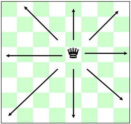
This freedom of movement is what makes the N-queens problem extremely hard.
Below is a short overview of how the remainder of this article progresses. We’ll discuss 4 different algorithms to solve the problem:
- The Brute Force solution.
- Backtracking based solution.
- Permutations based solution.
- Finally, the seemingly crazy solution using Bit Magic.
I would highly recommend reading through the solutions in this order. However, feel free to skip a solution if you’re already familiar with it.
The entire code for the solutions discussed below is available here.
The Brute Force Solution
while there is life on earth:
    try a possible arrangement of queens.

We’ve got an 8x8 chessboard, which means we have 64 different spots to place the queens. We need to calculate C(64, 8), or the number of combinations of 64 objects, taken 8 at a time.
C(n,r) = n! / (r!(n−r)!)
We get around 4.5 billion different combinations of placing the 8 queens on an 8x8 chessboard.
The brute-force algorithm is as follows:
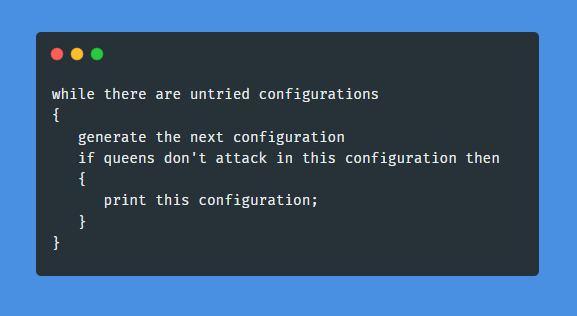
That’s a lot of permutations to check for a standard processor. We could use some sort of multi-processing solution (because checking one permutation is independent of another one).
But why do that when we have better algorithms to solve this problem?
Backtracking
We can do better than the naïve brute force solution for this problem. Consider the following pseudocode for the backtracking based solution:

The pseudocode looks simple enough, and you can checkout the python based code for this here. We won’t be looking at a description for the backtracking algorithm here.
I would however, like to discuss an optimization to reduce the time complexity of checking if we can place a queen in a cell on the board.
An important piece of the algorithm is where we have to check if a queen can be placed in a cell [i, j]. This step takes a long time. Let’s look at a brute-force way to do this, and then at an optimized version.
This has a time complexity of O(N), and this will be called multiple times for every cell on the board.
We can however, make use of some additional data structures to speed up the validity check for placing a queen on a cell [i, j]. This will bring down the complexity to O(1) — in other words, constant time. This is a huge reduction!.
The keys points in this piece of code are the following :
- All the elements in a particular diagonal (from left top to right bottom) have the same value for
row — column. - All the elements in a particular anti-diagonal (from right top to left bottom) have the same value for
row + column.
This optimization brings down the isSafe complexity to O(1). Hurray 😃.
Now that we’re done with the basic algorithms for N-Queens. Let’s move onto some more complicated ones that run much faster than the ones described above.
Permutations and N-Queens
The idea behind this algorithm is pretty simple. Consider the following facts about the placement of each queen:
- We can only place one queen in a row.
- Same thing can be said for each column.
- This means that all successful solutions are just going to be permutations of the column subscripts.
- Each successive row has one fewer candidate position for the queen to be placed.
Going by this logic, the problem space comes down to just 8! = 40,320.
That gives a lot less options to try and to find the solutions for our problem.
Let’s look at the pseudo-code for this approach:
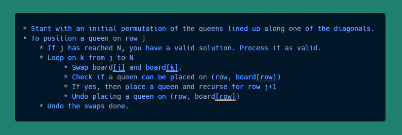
For greater clarity, let’s look at the code as well:
Note: board[i] stores the column number where a queen has been placed in row i. Hence, the cell value is given by (i, board[i]).
This optimization speeds up the calculation a lot, because of the highly reduced board space to consider while placing the queens.
The speed up becomes more prominent as we increase the size of the board, and hence the number of queens to be placed.
Also, the validity check for a particular cell becomes simpler, because now we only have to check diagonals and the anti-diagonals.
Let’s see some Bit Magic!
This particular solution to the problem is something that was practically Greek to me the first time I went through it.
That’s understandable though, because hey, it’s bit magic!
But thankfully, I found this amazing blog post explaining the entire algorithm line by line. The code is in JavaScript. I’ll be describing the same thing but for the code in python. Read whichever post suits you :)
The best way to go about explaining this algorithm is by putting up the code first 😉

The algorithm works using the same basic idea that was discussed before. We only need to check three things before placing a queen on a certain square:
- The square’s column doesn’t have any other queens on it
- The square’s left diagonal doesn’t have any other queens on it
- The square’s right diagonal doesn’t have any other queens on it
The code might look like a black box that just seems to work. That’s how I felt the first time I read this insanely fast piece of code.
Let’s try and break it down line by line.
Line #1
You’ll notice that the function accepts 4 parameters:
- column
- left_diagonal
- right_diagonal
- queens_placed
The queens_placed is self explanatory. We need to keep track of how many queens we have placed till now for the recursion to terminate at one point.
The three variables column, left_diagonal and right_diagonal are basically integers, but they are being treated as a sequence of bits for the purpose of this algorithm. These variables help us determine the open positions on the current row for a queen to be placed.
Let’s look at the picture below:
ld= left_diagonalcols= columnrd= right_diagonal
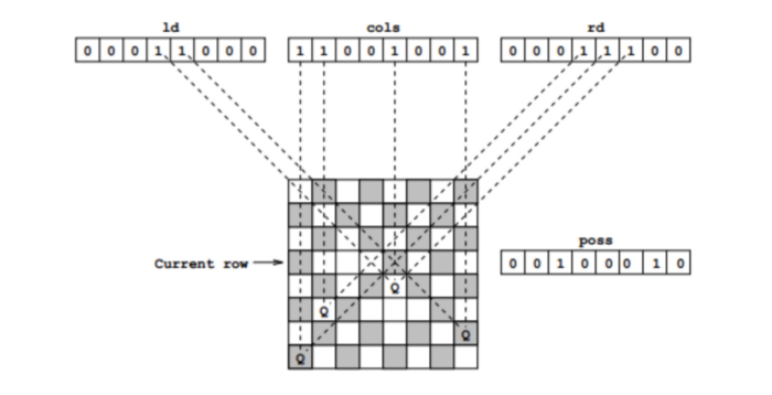
Ignore the poss variable for now. We’ll get to it later on.
Lines #2–6
These lines of code simply handle the base case for recursion. When we have placed N queens on our N by N board, we increment the number of solutions counter and print the solution if the appropriate flag has been set while running (see the entire code for this flag).
Line #8
This finds the valid_spots remaining on the current row. This is basically the poss variable depicted in the picture above.
valid_spots = self.all_ones &
~(column | left_diagonal | right_diagonal)
For example, let’s say that after some number of iterations we have:
left_diagonal = 00011000
column = 11001001
right_diagonal = 00011100
The code (column | left_diagonal | right_diagonal) just does an “OR” operation, and ends up with the bit sequence 11011101.
Then, adding the ~ in front of that expression causes the resulting bit sequence to “flip” (so all zeroes become ones and vice versa), and valid_spots would be set to 00100010.
So for the current row, the column number 0,1,3,4,5 and 7 are not available. We can only place a queen on column number 2 and 6. These are the only two spots that we will try.
Line #10
current_spot = -valid_spots & valid_spots
This line finds the first non zero bit and stores it into current_spot. So it’s basically finding the first empty spot where we can place our queen (from the rightmost column).
This right here is what makes the algorithm so fast. We used bit operators to directly tell us the empty positions that are completely safe for us to place our queens. Hence, this leads to major speedup as you will see later on.
Line #11 and 12
Line #11 simply adds the queen being placed at the current_spot to our solution set so that we can print it later.
Line #12 marks the current_spot as unavailable. Remember, XORing the same bits leads to 0.
Line #13
This is probably the most important line of code for this algorithm (and the most confusing one as well). Here we are just propagating the effects we introduced, further down to the next row.
We placed a queen at the current_spot and now we want to update our variables column, left_diagonal and right_diagonal to contain these changes as we move onto the next row.
self.solve((column | current_spot), (left_diagonal | current_spot)>> 1,(right_diagonal | current_spot) << 1, queens_placed + 1)
Note: a | b means bitwise OR for variables a and b. Also, a « 1 is a left-shit operator. Similarly, a » 1 is the right-shift operator.
So calling (right_diagonal | current_spot) << 1 simply says: combine right_diagonal and current_spot with an OR operation, then move everything in the result to the left by one.
For example — say right_diagonal had value 00011100. And say we made the queen occupy the last slot such as the last 1 in the valid_spots integer 00100010.
Then the current_spot would become 000000010 and OR-ing it with the right_diagonal would give us 00011110. We left-shift it to get 00111100 and that is exactly the effect we want for the right-diagonal.
The right-diagonal is moving from right top to bottom left. Left-shift on the bits produces that effect.
For a greater clarity, try doing this operation on a paper:

We start with 0s for all the three variables, meaning that all the positions are available in the first row for placing the queens.
Now comes the fun part (well, something to amaze you 😆), Speed Comparisons.
Stats
Let’s look at the stats for a tool that Google built for solving the N-Queens.
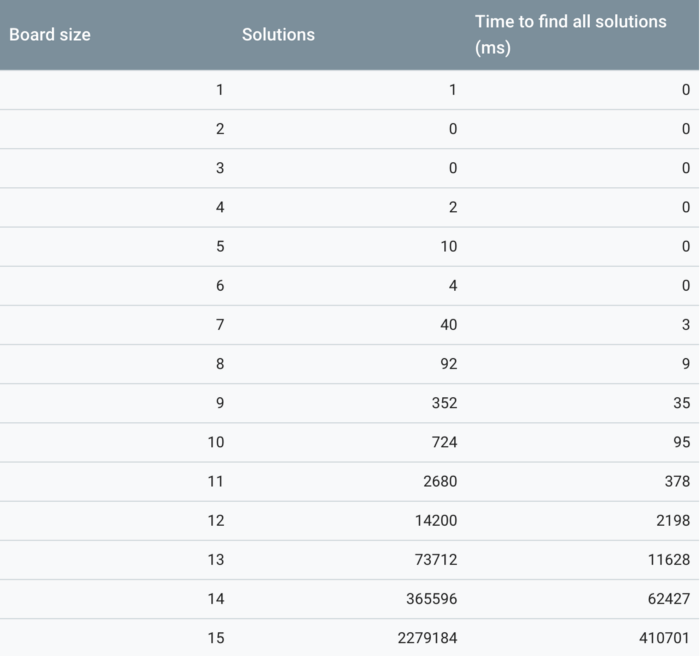
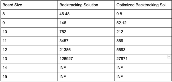
Following are the stats for the 4 different approaches we discussed for the N-Queens:
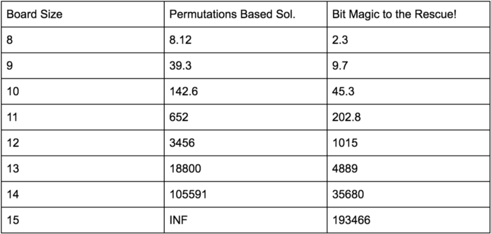
The last solution involving bitwise operators clearly performs better than the results reported by the Google’s N-Queens solver. 😃
Also, an interesting thing to note here is the effect that slight optimization had on the results. Recall the optimization where we converted the is_cell_safecheck from an O(N) solution to an O(1) check. This clearly shows us how such small changes can bring about huge performance impacts.
If you’ve read along till the very end, I’m sure your algorithmic curiosity has now been satisfied! But hey, this is just the tip of the iceberg 😉.
I have another post coming up soon where we’ll tackle a problem similar to the N-Queens but with a slight twist.

Leave a comment